Turbulence Dissipation Rate in the Atmospheric Boundary Layer
While simulations of the atmosphere are carried out at finer and finer resolution, our representations of the details of turbulence (especially its breakdown or dissipation) have not kept pace. We are very interested in measuring turbulence dissipation rate in situations like frontal passages (JAS2004), in wind turbine wakes (BLM2015), on towers extending up to 300-m (MWR2018, AMT2018), in complex terrain (AMT2019), and offshore (GRL2019). Some of our measurements use conventional sonic anemeometers, but we also use a tethered lifting system for wind turbine wake measurements at NREL and in the Perdigão field campaign (AMT2019b), as well as lidars (JTech2013, AMT2018). Using machine learning (GMD2020), we are exploring how to improve modeling of TKE dissipation rate!
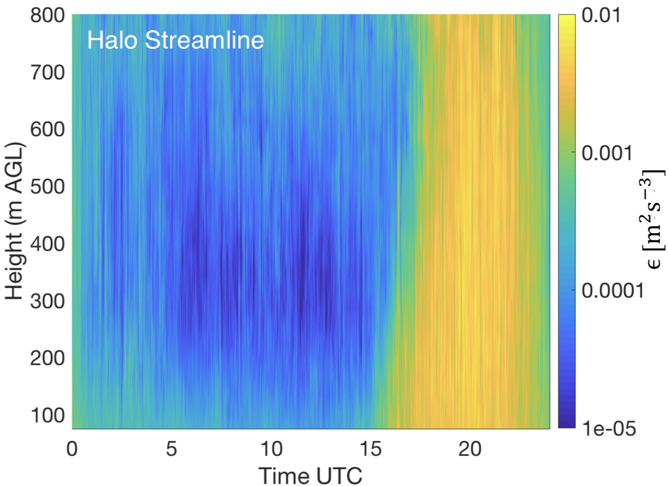 Figure Caption: Daily
climatology of turbulence dissipation rate derived from raw values from
the Halo Stream Line lidar during the XPIA field campaign at the
Boulder Atmospheric Observatory. From AMT2018.
Figure Caption: Daily
climatology of turbulence dissipation rate derived from raw values from
the Halo Stream Line lidar during the XPIA field campaign at the
Boulder Atmospheric Observatory. From AMT2018.
Detailed Observations of Complex Flow due to Wind
Turbine Wakes
We utilize profiling lidar (JTech 2012, BLM2013, AMT2015), scanning lidar (JTech 2013, JRSE 2014, JTech 2014a, JTech2014b, AMT2017),
radiometers (GRL 2012), meteorological towers (ERL2012, JSEE 2013) and tethered lifting systems (BLM2015)
to study the development and propagation of wind turbine wakes in different atmospheric conditions, with
special interest in wind farms co-located with agriculture (BAMS 2013, AFM 2014) and in complex terrain (AMT2019b).
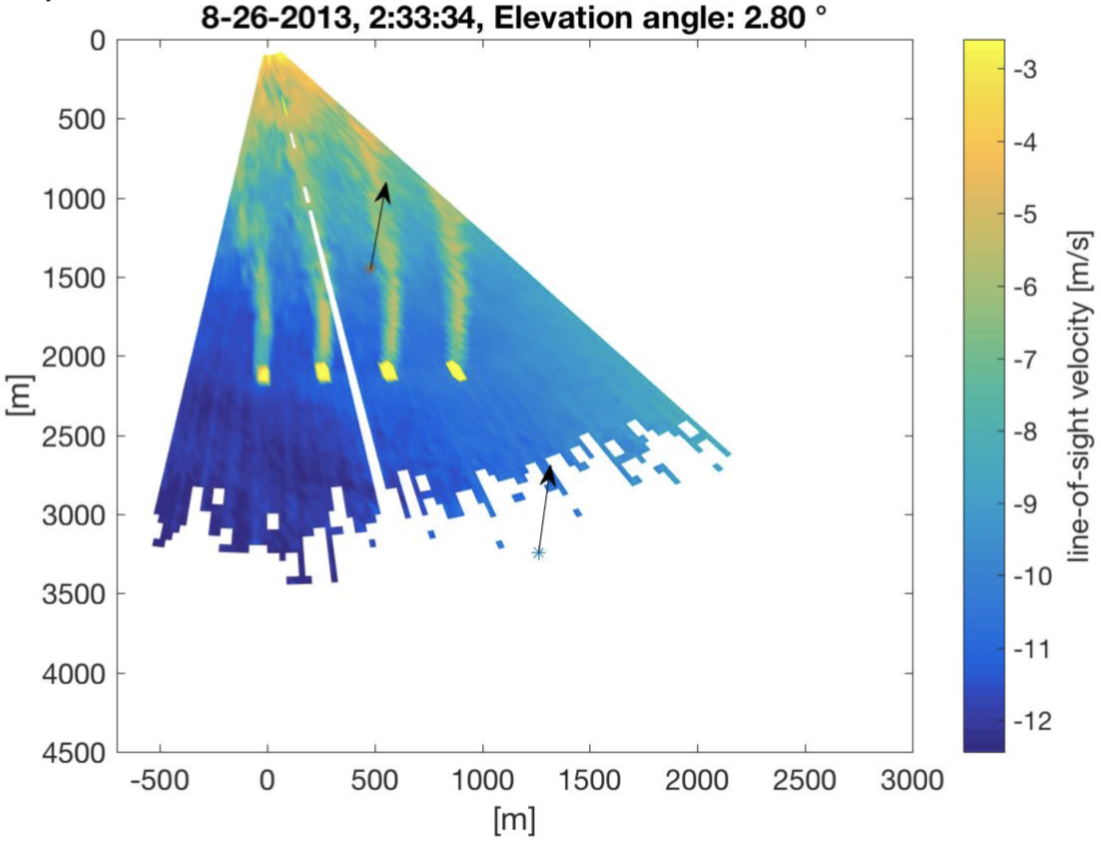 Figure Caption: Wakes
from four turbines in the CWEX-13 campaign. Color maps of line-of-sight
velocity measured by the scanning lidar during a PPI scan performed at
11:57 UTC (06:57 LDT)
Figure Caption: Wakes
from four turbines in the CWEX-13 campaign. Color maps of line-of-sight
velocity measured by the scanning lidar during a PPI scan performed at
11:57 UTC (06:57 LDT)
on 23 August 2013. The scanning lidar is located in the origin of the
coordinate system. The two arrows show wind direction as measured by
the profiling lidars WC-1 and WC-2 at 80 m above ground level. From AMT2017.
Large Eddy Simulations of the Atmospheric Boundary Layer & Nesting LES within Mesoscale Simulations
Improved turbulence models (MWR 2010b) and/or immersed boundary methods (MWR 2010a, MWR 2012) may be required to simulate complex flow in stable atmospheric boundary layers or in regions of complex terrain. To elucidate interactions of atmospheric stability with wind turbine wakes, large-eddy simulations with a generalized actuator disk model (JRSE 2014a, JRSE 2014b) or actuator line model (JRSE2017) demonstrate how ambient turbulence accelerates the erosion of wind turbine wakes. Instrument simulators in LES can also help characterize instrumental uncertainty (AMT2015) and assess how hurricanes may impact wind turbines (GRL2017). When nesting LES within mesoscale simulations, caution must be used in selecting resolutions (JAMES2017) and mesoscale forcings (JPhys2017) even as such nesting can provide better agreement with observations (MWR2018). We have developed and tested new methods of "tickling" up turbulence in nested LES (JAMES2019). LES of a wind turbine wake have been used to demonstrate that wind turbine wakes do not pose hazards to small aircraft (WES2018a).
Offshore Wind Energy
While offshore wind energy is well-developed in Europe, North
American has few offshore wind farms and a lack of data characterizing
our marine wind resource (BAMS2014). Hurricanes will challenge offshore wind turbines here, but large-eddy simulations of hurricanes (BLM2017a, BLM2017b) can provide important assessments of turbulence characteristics for wind turbine design (GRL2017) and loads estimation (WES2020a). Measurements of wakes from European offshore wind farms are consistent with our mesoscale simulations of wind farms (MetZeit2018, ERL2018, GMD2020). The
few measurements available offshore of North America suggest that
offshore wakes will be strong and persist for long distance (GRL2019).
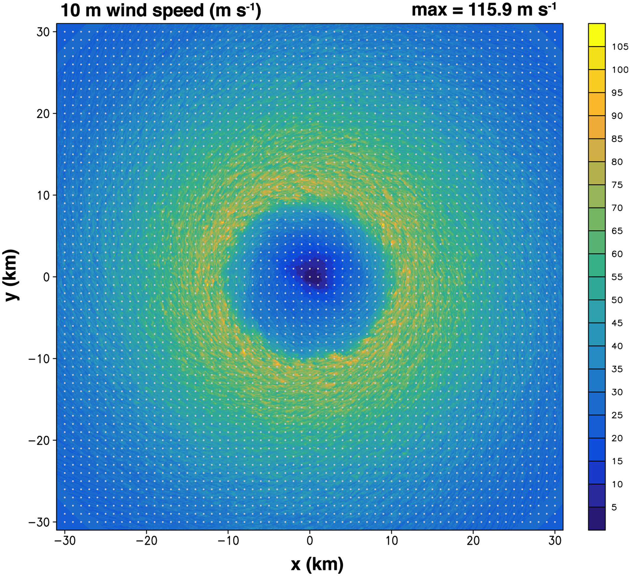 Figure Caption: Large-eddy
simulations of a Category 5 hurricane: Instantaneous snapshot of the
10-m wind field produced by the CM1 model (∆x = ∆y = 31.25 m).
Locations of virtual towers used for analyzing data for turbine
response are shown as the gray dots. From GRL2017.
Figure Caption: Large-eddy
simulations of a Category 5 hurricane: Instantaneous snapshot of the
10-m wind field produced by the CM1 model (∆x = ∆y = 31.25 m).
Locations of virtual towers used for analyzing data for turbine
response are shown as the gray dots. From GRL2017.
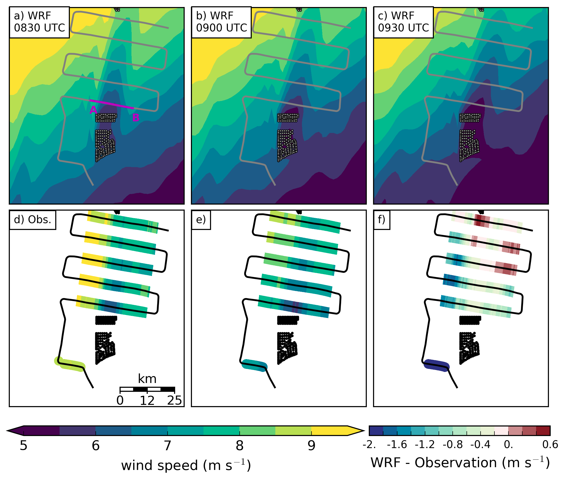 Figure Caption: Comparison of simulated and measured wind speed at hub height in the far field of the wind farm. The simulated wind speed at
hub height during the observational period (a) 0830, (b) 0900 and (c)
0930 UTC is shown in colored contours. The observed wind speed
at hub height is shown in (d) in the same colored contours as the
simulation results (e). The black line denotes the flight track. Black
dots
indicate the locations of the single wind turbines. In (e) the
simulation results were interpolated onto the flight track, spatially
and timely,
for details – see text. In (f) the difference, WRF (e) − observation
(d) along the fight track is plotted. The vertical cross section shown
in
Figure 8 is shown by a pink line, with the beginning and end of cross section annotated with A and B, respectively. From MetZeit2018.
Atmospheric Impacts on Wind Energy
Production
Atmospheric stability impacts wind turbine power production sometimes in contradictory ways (Wharton & Lundquist ERL 2012 vs Vanderwende & Lundquist ERL 2012)
depending on local meteorology, but refined measurements of both wind shear and wind veer explain this difference (WES2020b). Neural networks can extend limited
measurements at a site towards improved resource assessment (ERL 2013). Detailed lidar observations and WRF simulations of nocturnal low-level-jets (LLJ) (MWR 2015) suggest that LLJ-induced wind shear and veer extend into the
turbine rotor-layer during intense jets. Ramp events, in which winds
rapidly increase or decrease in the rotor-layer, were also commonly
observed during jet formation periods. At large spatial scales, we
evaluate the statistical independence of wind generators, and find that
higher-rate fluctuations in wind power generation can be effectively
smoothed by aggregating wind plants over areas smaller than otherwise
estimated (ERL2015). New approaches to maximizing power production by steering wakes (WES2019) are more beneficial during stably stratified conditions.
Mesoscale Modeling of Wind Farms
To
assess the local and regional impacts of wind energy development, we
have implemented a wind farm parameterization into the Weather Research and Forecasting model.
The Fitch et a. parameterization (MWR2012a, MWR2012b)
is available with every WRF download since version 3.3. In simulations
of the CASES-99 GABLS case, the wind farm wake varies throughout the
diurnal cycle, with the maximum downwind surface temperature increases
~ 0.5K at night (MWR2013) consistent with observations. Comparisons between this
elevated drag model and climate simulations representing wind farms
simply with enhanced surface roughness show nearly the opposite local
impacts on surface temperature (JClim2013). We have evaluated the skill of the WRF WFP in comparison to large-eddy simulations of a small wind farm (JAMES2016) and in comparison to onshore wind farm power production (GMD2017). Wind farms can interact with each other, causing economic impacts due to wake wind speed deficits (NE2018). And, wind farms can even affect meteorological phenomena like thunderstorm outflow (WES2020)! When simulating wind farms in a mesoscale model, modeling choices are critical (GMD2020).
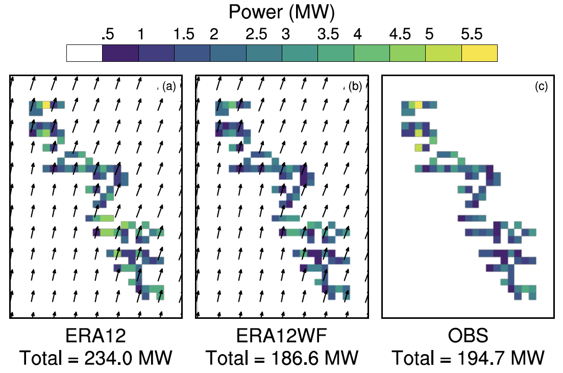
Figure Caption: Simulating
observed power production at an onshore wind farm. Here we see the
power production for one 10 min period from the WRF simulation with
12-m vertical resolution and ERA-Interim boundary conditions (a), the WRF simulation with the Wind Farm Parameterization with 12-m vertical resolution and ERA-Interim boundary conditions
(b), and the observation (abbreviated as OBS) (c). The total power in
each grid cell is presented regardless of the number of turbines in
each cell, and the wind-farm totals are summarized at the bottom. The
vectors indicate the simulated winds, and their lengths correspond to
the horizontal velocity magnitude. From GMD2017.
Wind Farms and Society
LES of a wind turbine wake have been used to demonstrate that wind turbine wakes do not pose hazards to small aircraft (WES2018). Wind farms generate wakes that impact other wind farms' inflow wind speed and power production, during certain wind speed, direction, and atmospheric stability regimes (NE2018), suggesting that more coordinated planning of wind farms could benefit society's use of wind energy.
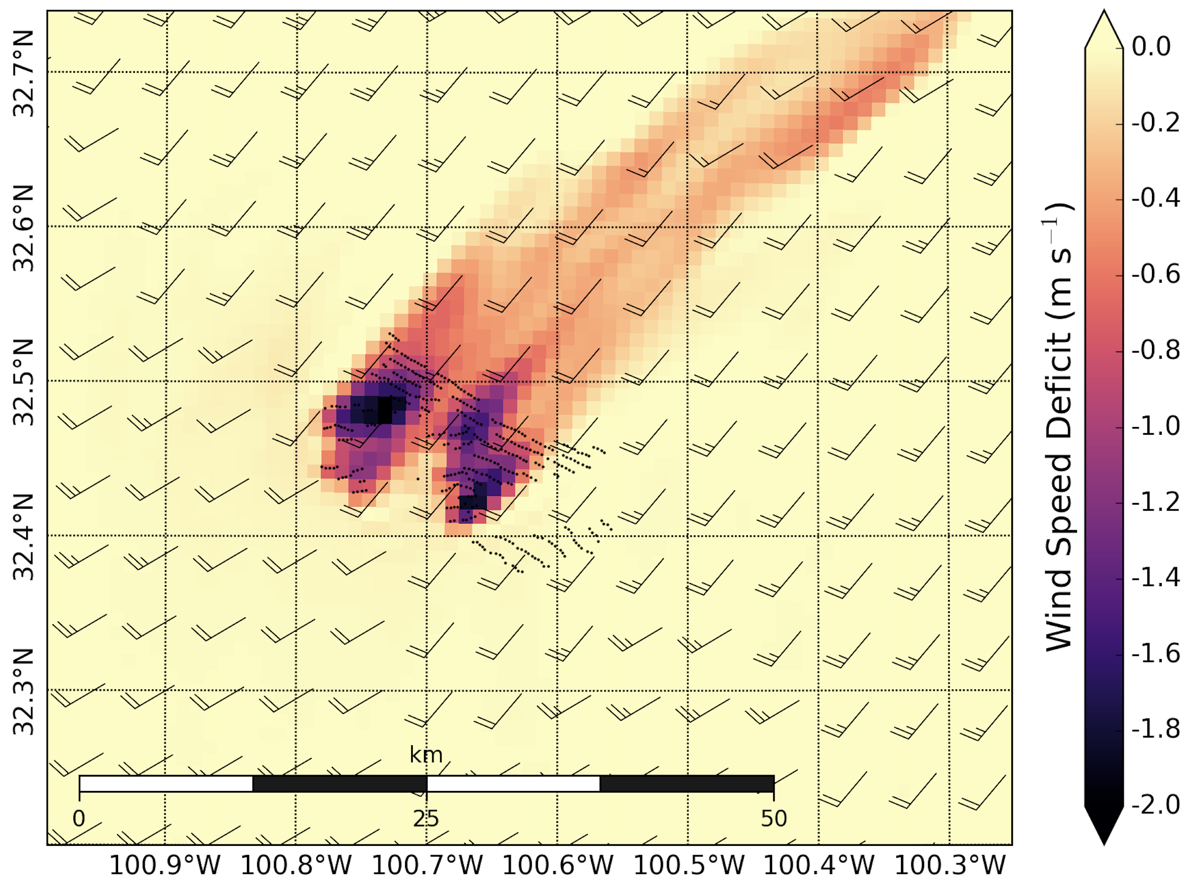 Figure Caption: Wake
wind speed deficit as simulated by WRF with the wind farm
parameterization at a complex of wind farms in West Texas for 0200 UTC
(2100 LST) on 24 January 2013. The domain is large, ~ 70 km x
50km, and the grid cells denote 0.1-degree changes in latitude
and longitude, with wind barbs showing the 80-m wind speed and
direction for that cell. The 1-km grid cells can be seen in the pixels
of the wind speed deficits, which show the upwind farm’s wind farm wake
at an 80-m altitude extending more than 50 km downwind and clearly
impacting the winds at the downwind farm. From NE2018.
Figure Caption: Wake
wind speed deficit as simulated by WRF with the wind farm
parameterization at a complex of wind farms in West Texas for 0200 UTC
(2100 LST) on 24 January 2013. The domain is large, ~ 70 km x
50km, and the grid cells denote 0.1-degree changes in latitude
and longitude, with wind barbs showing the 80-m wind speed and
direction for that cell. The 1-km grid cells can be seen in the pixels
of the wind speed deficits, which show the upwind farm’s wind farm wake
at an 80-m altitude extending more than 50 km downwind and clearly
impacting the winds at the downwind farm. From NE2018.
Wind Farms and Climate
While there is uncertainty with the details of how climate change will affect wind resources, using ensembles of climate models can help provide some indications as well as uncertainty quantification (NG2018). Wind energy is currently a small part of our electricity portfolio, but modeling tools can predict the small local changes introduced by wind farms (JClim2013, GMD2017)
Fire Meteorology
In a changing climate, wildfires occur more frequently and may have
higher intensities. Using WRF-Fire, we investigate smoke dispersion and
impacts on local and regional weather and climate.
Urban Meteorology
Cities can create their own microclimates with interesting implications for detailed simulations of flow in urban areas (JAMC 2007; JAMC 2008) and air pollution events (JAMC 2013), especially when urban meteorology interacts with nocturnal low-level jets (LLJ). Immersed boundary methods may be required for simulations in urban areas (MWR 2010, 2012).